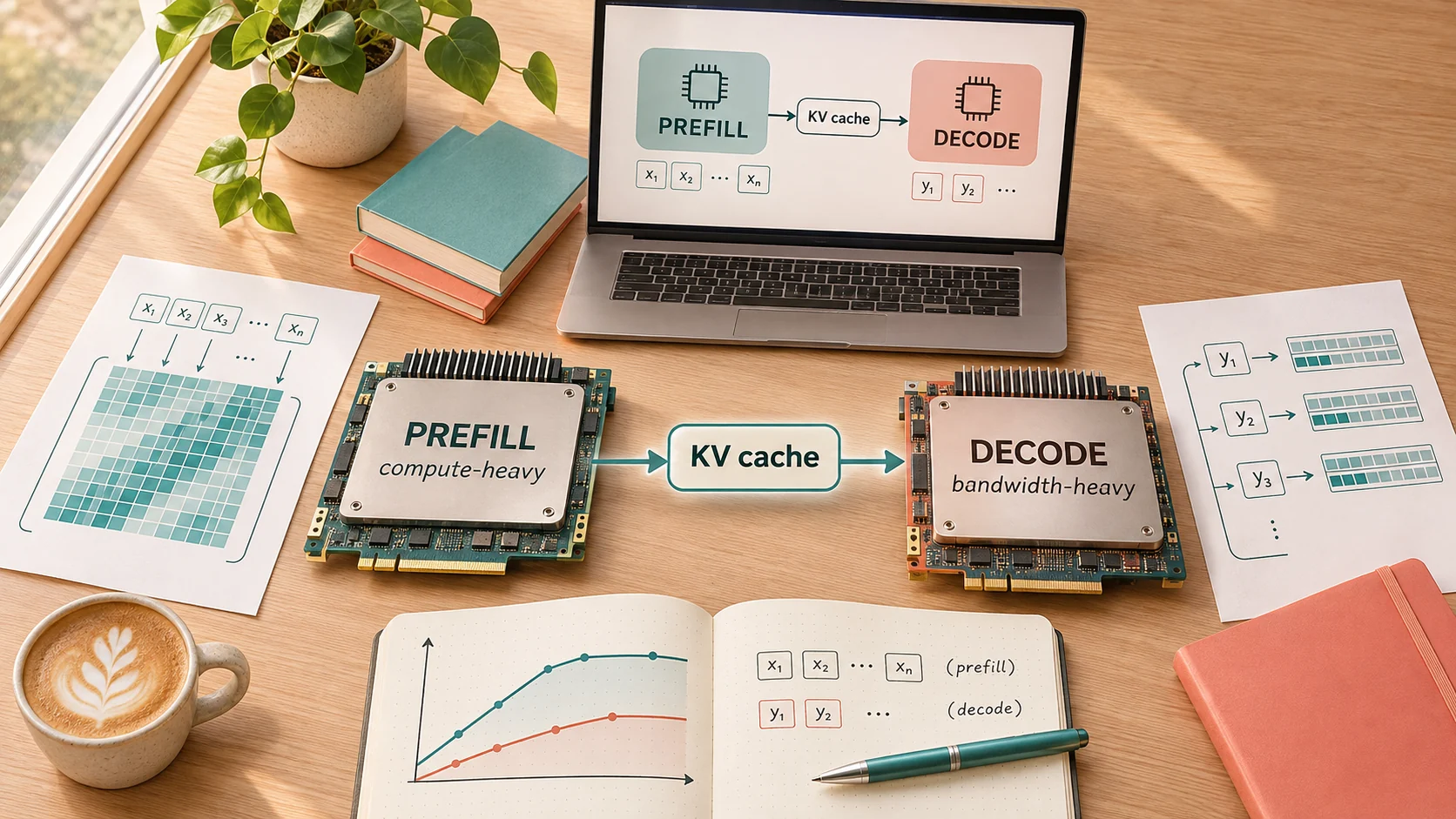
The idea sounds simple: process the prompt on a chip built for compute, then hand generation to a chip built for memory bandwidth. Nvidia and AWS have both built products around it. The part the architecture diagrams leave out is what has to cross between the two chips. For a long prompt, the state produced during prefill can be several gigabytes per request, and Nvidia's own platform offers more than one place to draw the line. I read this as a question about where to put the boundary in an inference system. Splitting is worth it when the time it saves in queueing and per-token latency exceeds the transfer time it exposes, with both fleets kept busy and at the same cost.
What each phase asks of the hardware
Prefill processes the whole prompt in one pass. Each weight loaded from memory is applied to every prompt token, so a long prompt performs many floating-point operations for each byte the chip moves. A long, dense prefill often runs close to the chip's compute limit. Short prompts, small chunks, and attention over very long contexts can change that, so prefill is not compute-limited in every case.
Decode produces one token per sequence per step. In a simple weight-streaming picture, each step touches most of the model weights. For a model stored in BF16 that is about 2 FLOPs for every 2 bytes of weights, or about 1 FLOP per byte at batch size 1, before counting reads of the KV cache.
An H100 SXM delivers 989 TFLOP/s of dense BF16 compute and 3.35 TB/s of HBM bandwidth [3]. The ratio, about 295 FLOPs per byte, is the ridge of the roofline: below it a kernel is limited by memory bandwidth, above it by compute. Batch-1 decode sits near 1 FLOP per byte in this model, so at low batch sizes the sustained bandwidth for weights and the KV cache usually limits throughput.
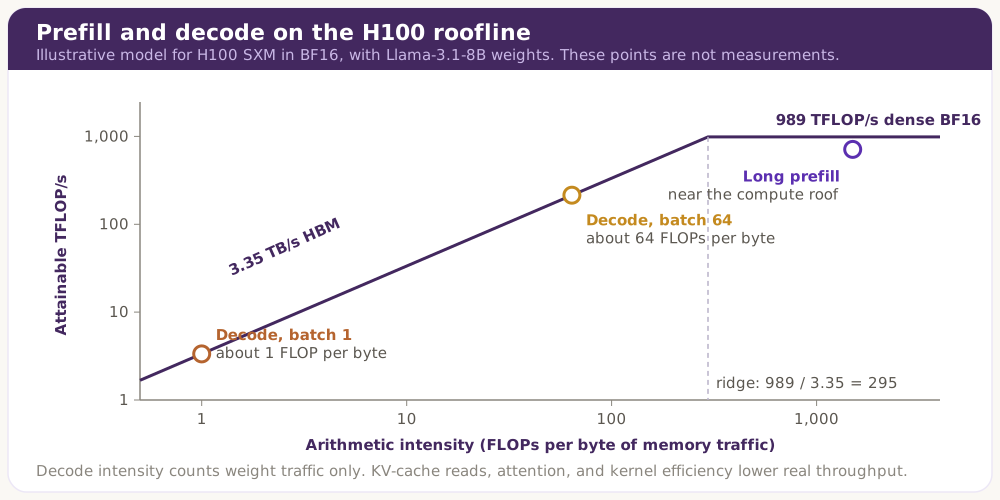
Fig. 1 — An illustrative roofline for Llama-3.1-8B on an H100 SXM, built from the published peak compute and bandwidth. The points are not measurements. They count weight traffic only, so KV-cache reads, attention, and kernel efficiency place real decode lower.
Batching is the standard fix for decode. When 64 sequences decode together, one read of the weights can serve all 64, which moves decode toward 64 FLOPs per byte in this model. That is still below the ridge on an H100, and each added sequence brings its own KV cache, which also has to be read every step. I wrote about that growth in the KV cache post, and I explain the roofline in two IBM Technology lightboard videos, The AI Memory Wall and The KV Cache Effect.
Why the phases interfere on one pool
On a shared pool, a long prefill occupies the accelerators and can delay the decode steps of other requests in the batch, which raises their time per output token. Giving decode priority instead delays the first token of new requests. Modern single-pool schedulers reduce this conflict. Sarathi-Serve splits each prefill into near-equal chunks and adds new requests to a batch without pausing ongoing decodes [4]. Chunked prefill and continuous batching are the baseline a split design has to beat.
Research systems have measured what separating the phases can gain. DistServe gives prefill and decode their own GPUs and tunes resources and parallelism for each phase; in the authors' experiments it served 7.4 times more requests, or met latency targets 12.6 times tighter, than the systems it was compared with [5]. Splitwise ran the phases on separate machines and reported 1.4 times higher throughput at 20 percent lower cost [6]. Mooncake, the serving platform behind Moonshot AI's Kimi, separates prefill and decode clusters and pools the KV cache across CPU memory and SSD; the authors report that under real workloads it lets Kimi handle 75 percent more requests [7]. Each of these results comes from its own models, hardware, baselines, and latency targets, so the numbers show that disaggregation can help. They do not rank the systems against each other.
Three places to put the boundary
Those research systems split the phases across GPUs of the same kind. In 2026 the second side became a different chip, and the boundary started to move.
AWS pairs Trainium3 for prefill with Cerebras CS-3 systems for decode, connected over its Elastic Fabric Adapter network [2]. The full KV cache crosses once per request. Cerebras states that the WSE-3 holds the model in 44 GB of on-chip SRAM with 21 PB/s of bandwidth [10].
Nvidia's Vera Rubin platform with the Groq 3 LPX supports three execution modes [1]. In the first, Rubin GPUs run prefill and hand the KV cache to the LPX once per turn, and the LPX runs the whole decode step. In the second, the split happens inside decode: Rubin GPUs compute attention and keep the KV cache, the LPX runs the feed-forward and mixture-of-experts layers, and only intermediate activations cross between racks, once per full-attention layer. In the third, the LPX runs a small draft model for speculative decoding, and only draft tokens cross. Nvidia's March architecture post centers on the attention and feed-forward split [8]. Nvidia says each LPU has 500 MB of on-chip SRAM, and its Ian Buck told IEEE Spectrum that the LPU has seven times the memory bandwidth of the GPU [9]. Nvidia gained the technology through a non-exclusive license and by hiring Groq's founder and other staff in December 2025; Groq continues as an independent company [11].
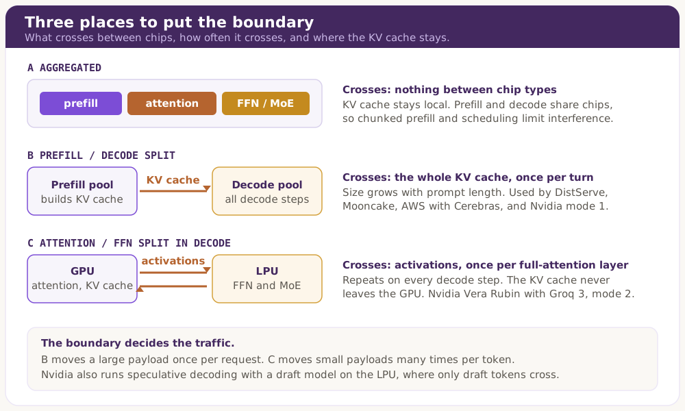
Fig. 2 — Layout B moves a large payload once per request, and layout C moves small payloads many times per generated token. The choice of boundary sets the size and frequency of the traffic and the scheduling problem that comes with it.
On-chip SRAM does not remove the memory question. SRAM capacity is small next to HBM, so a long-context workload can exceed what a decode chip holds locally, and the model's layout across many chips and their interconnect then matters. The vendor bandwidth figures also come from different measurement scopes and are not directly comparable with H100 HBM bandwidth.
The cost of moving the KV cache
In layout B the KV cache crosses the network before the first output token. For Llama-3.1-8B, which has 32 layers and grouped-query attention with 8 key-value heads of dimension 128 [12], keys and values in BF16 take 2 × 32 × 8 × 128 × 2 bytes, or 128 KiB per token. A prompt of 32,768 tokens carries a 4 GiB KV cache. At the full line rate of a 400 Gb/s link, 50 GB/s, moving it takes about 86 milliseconds.
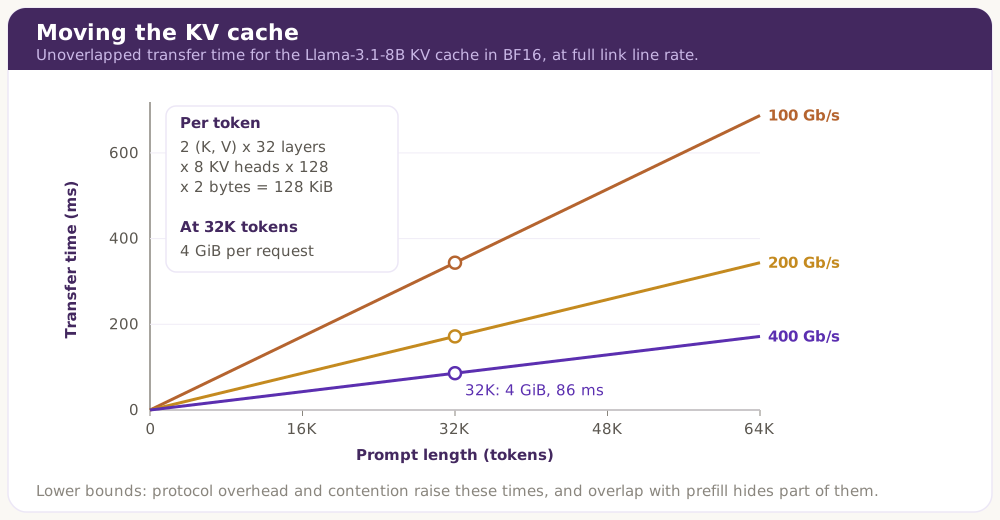
Fig. 3 — Unoverlapped transfer times at full link line rate, which makes them lower bounds. Protocol overhead and network contention raise them. Streaming the cache layer by layer during prefill hides part of them. Compression and prefix reuse reduce the bytes.
Systems hide part of this cost. They can stream the cache layer by layer while prefill is still running, and DistServe places the two phases according to the cluster's bandwidth to limit the traffic [5]. Mooncake keeps a shared KV store, so a repeated prompt prefix does not have to be recomputed or sent again [7]. Neither AWS nor Cerebras has published the transfer latency of their combined system.
Prompt length cuts both ways. A 2,048-token prompt moves in about 5 milliseconds at this ideal rate, but it also gives a dedicated prefill pool little work. A 32K-token prompt has enough prefill work to justify specialized hardware and also carries 4 GiB across the network. Neither the prompt length nor the link speed decides the outcome alone.
Where the time goes
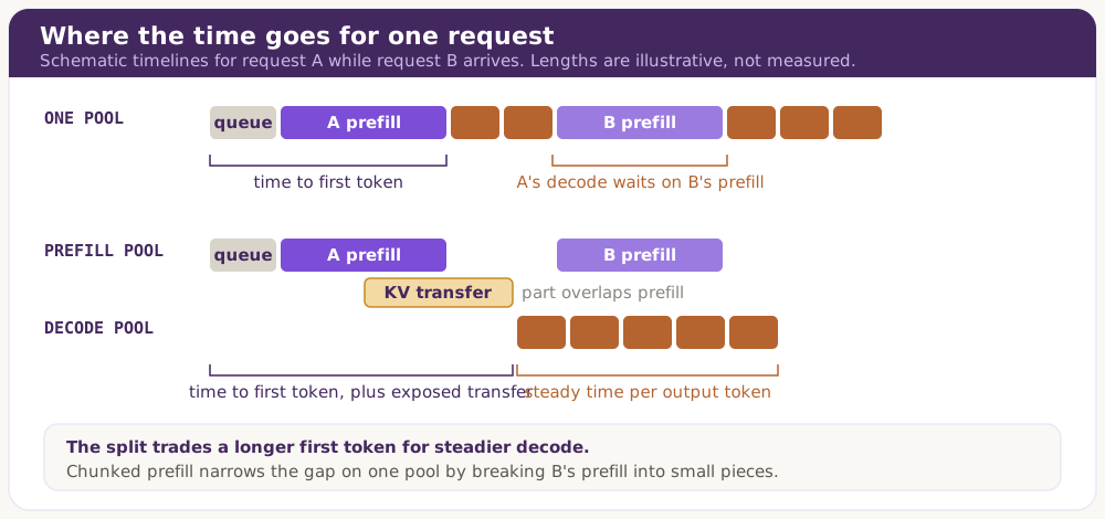
Fig. 4 — The prefill and decode split usually trades a longer time to first token for steadier time per output token. On a single pool, chunked prefill narrows the gap by breaking B's prefill into small pieces.
Time to first token and time per output token have to be compared separately. A split design can improve one and worsen the other, and whether the number of requests served within both targets rises depends on the request mix.
Deciding per request: llm-d
The commercial systems above make the split a property of the hardware. llm-d, an open-source serving stack for Kubernetes that runs on vLLM and SGLang, makes it a decision for each request. Its router can send a request's prefill to a pool of prefill workers and its decode to a pool of decode workers, with the KV cache moved between them by NVIDIA's NIXL library over RDMA [13].
The router does not split every request. It chooses the decode worker first and then checks two thresholds. If the prompt is shorter than a configured length, the whole request runs on the decode worker. Disaggregation happens only when the part of the prompt missing from the prefix cache reaches a second threshold, and then prefill runs on a separate worker [13]. That is the break-even test from the opening, applied one request at a time. Workers are chosen by prefix-cache match and load, so a request also tends to land where its shared context is already stored.
The deployment guide states that "NIXL works over TCP, but RDMA networking (InfiniBand, RoCE, EFA) is highly recommended for production" [14], which matches the transfer cost in Fig. 3. Red Hat launched llm-d in May 2025 with CoreWeave, Google Cloud, IBM Research, and NVIDIA as founding contributors [15], and the project reached version 1.0 in October 2026 [16]. IBM, where I work, is one of its lead maintainers, along with Red Hat and Google [16].
Deciding whether to split
The break-even test from the opening can be written out. The exposed penalty of a split is the transfer and coordination time that overlap does not hide. The split is promising when the queueing and service time it saves is larger than that penalty, at the same cost and with both fleets kept busy. That last condition is easy to miss. Two pools that are each efficient can still strand hardware when the ratio of long-prompt to long-output requests shifts during the day.
These are the measurements I would ask for before choosing an architecture:
- Traffic shape: the full distributions of prompt and output lengths, the number of active sequences, prefix reuse, and how bursty the arrivals are.
- Latency: time to first token and inter-token latency at the median and the 95th or 99th percentile, and total request time.
- Utilization: compute use on the prefill side, memory bandwidth and occupancy on the decode side, queueing time, bytes of KV cache moved, and idle capacity on both fleets.
- Outcome: requests per second served within the latency targets, and energy and cost per request.
Vendor figures need the same scrutiny. Cerebras expects a disaggregated Trainium and Cerebras system to raise token throughput 5 times over an aggregated one, and presents that as a projection without supporting data [10]. Nvidia reports 3,431 tokens per second for Gemma 4 31B on Groq 3 LPX at 100K input tokens, measured by Artificial Analysis [1]. A measured benchmark, a vendor statement, and a projection are three different kinds of evidence.
My take, from the systems side
I would not choose a disaggregated design from a tokens-per-second headline. I would start with the prompt and output length distributions, the tail latencies the application cares about, and the bytes that cross the hardware boundary. Then I would profile a strong single-pool baseline, with chunked prefill and continuous batching, against the split design under the same latency targets and cost. For mixed traffic with short prompts, the single pool can be the better choice, and IEEE Spectrum notes that a Cerebras WSE-3 can also run inference alone [9]. The new chips give architects more places to put the boundary, and each one has to be measured.
Several of these papers are on the reading list of my Scaling LLMs seminar at Columbia, and the question my students return to most is what was measured, and on which traffic. Now that heterogeneous systems are sold as cloud products, that question also has to be asked about the boundary between the chips.
References
[1] NVIDIA, "How NVIDIA Groq 3 LPX Unlocks Ultrafast Interactivity at Long Context on NVIDIA Vera Rubin," NVIDIA Technical Blog, August 24, 2026.
[2] Cerebras, "AWS and Cerebras Collaboration Aims to Set a New Standard for AI Inference Speed and Performance in the Cloud," March 13, 2026.
[3] NVIDIA, "NVIDIA H100 Tensor Core GPU," product specifications. The dense BF16 figure is half the listed 1,979 TFLOP/s, which assumes sparsity.
[4] Amey Agrawal et al., "Taming Throughput-Latency Tradeoff in LLM Inference with Sarathi-Serve," 2024.
[5] Yinmin Zhong et al., "DistServe: Disaggregating Prefill and Decoding for Goodput-optimized Large Language Model Serving," OSDI 2024.
[6] Pratyush Patel et al., "Splitwise: Efficient Generative LLM Inference Using Phase Splitting," ISCA 2024.
[7] Ruoyu Qin et al., "Mooncake: A KVCache-centric Disaggregated Architecture for LLM Serving," FAST 2025.
[8] NVIDIA, "Inside NVIDIA Groq 3 LPX: The Low-Latency Inference Accelerator for the NVIDIA Vera Rubin Platform," NVIDIA Technical Blog, March 16, 2026.
[9] Matthew S. Smith, "The AI Inference Revolution Is Here," IEEE Spectrum, September 15, 2026.
[10] Sarah Chieng, "The GPU Is Being Split in Half," Cerebras, March 26, 2026.
[11] Groq, "Groq and Nvidia Enter Non-Exclusive Inference Technology Licensing Agreement to Accelerate AI Inference at Global Scale," December 24, 2025.
[12] Meta, "Llama-3.1-8B model card," Hugging Face.
[13] llm-d, "Disaggregated Prefill/Decode," llm-d router documentation, GitHub.
[14] llm-d, "Deploy Prefill/Decode Disaggregation," llm-d well-lit paths documentation.
[15] Red Hat, "Red Hat Launches the llm-d Community, Powering Distributed Gen AI Inference at Scale," May 20, 2025.
[16] Peter Hess, "llm-d 1.0 hardens open-source AI inference for day 2 production operations," IBM Research, October 20, 2026.
Discussion
Sign in with GitHub to leave a comment or react. Threads are public and live in this site's GitHub Discussions.