
Back to home
Dataflow Architectures for AI specialization logo

Dataflow Architectures for AI

Six online courses, taught by Dr. Kaoutar El Maghraoui

AI accelerators run the same model in different ways, and those differences decide how fast it runs and how much it costs. This specialization follows one PyTorch model from graph capture through compilation, memory placement, debugging, and performance analysis on NVIDIA GPUs, Google TPUs, the Cerebras Wafer-Scale Engine, the Groq LPU, and IBM Spyre.

Scan to open on Coursera
QR code that opens the Dataflow Architectures for AI specialization on Coursera

coursera.org/specializations/dataflow-architectures-for-ai

6 courses
on Coursera, from IBM
6 labs
hands-on PyTorch in Google Colab
About 30 hours
at an intermediate level
Certificate
AI Systems Performance Engineering

What happens below the framework

Most engineers write a model in PyTorch and never see what the accelerator does with it. The six courses cover that hidden part: how the compiler turns the model into kernels, how the hardware schedules the work, where the data lives, how to debug a wrong answer, and how to predict and measure speed.

All five accelerators are studied with one common systems framework, so the comparisons carry over to new hardware. Topics include dataflow execution, TorchInductor, XLA, compiler scheduling, memory hierarchies, KV-cache behavior, numerical debugging, and roofline-based performance modeling.

The specialization is for ML engineers, compiler engineers, hardware architects, researchers, and advanced students. You should be comfortable with Python, neural networks, and basic computer architecture.

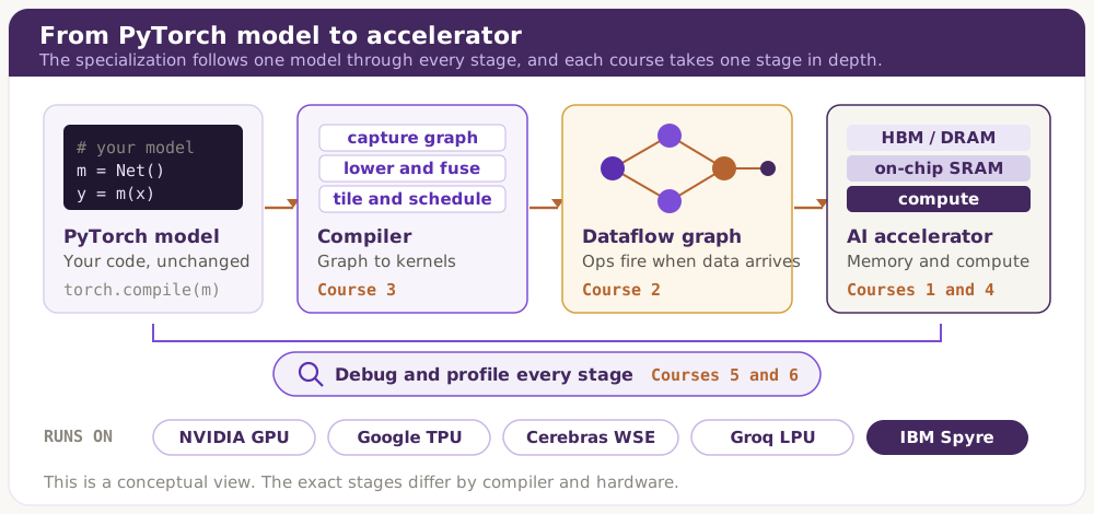
Pipeline from PyTorch model to accelerator. A PyTorch model goes to the compiler (capture graph, lower and fuse, tile and schedule, Course 3), then to a dataflow graph where ops fire when data arrives (Course 2), then to an AI accelerator with HBM or DRAM, on-chip SRAM, and compute (Courses 1 and 4). A bar below spans all stages: debug and profile every stage, Courses 5 and 6. The targets are NVIDIA GPU, Google TPU, Cerebras WSE, Groq LPU, and IBM Spyre.
Each course takes one stage of the path from a PyTorch model to the accelerator, and the last two courses cover debugging and performance across all of them.
“By the end of the course, when you see a new AI accelerator, I want you to know what questions to ask about it. What's the execution model? Where is the memory? Who schedules the operations? What does the compiler control?”
Dr. Kaoutar El Maghraoui, in IBM Research, October 2026

Courses in order

Each course builds on the ones before it, and each one has its own Coursera page.

The Accelerator Landscape course logo
Course 1 4 to 4.5 hours

The Accelerator Landscape

NVIDIA GPUs, Google TPUs, Cerebras, Groq, and IBM Spyre all run neural networks, but each makes different choices about how work is scheduled and where data is kept. The course compares those choices with one framework built on Amdahl's law, arithmetic intensity, and the roofline model.

Lab: Profile LLM inference on a CPU and a GPU, place the measurements on a roofline, and start an Accelerator Landscape Map that you extend in every later course.

  • Explain why AI workloads benefit from domain-specific accelerators using Amdahl's law and arithmetic intensity.
  • Compare execution and memory models across GPU, TPU, Cerebras, Groq, and IBM Spyre.
  • Use a roofline model to tell compute-bound from memory-bound workloads.
View on Coursera
Dataflow Execution Models course logo
Course 2 5.5 to 6 hours

Dataflow Execution Models

In a dataflow machine an operation runs when its inputs are ready. The course covers static and dynamic scheduling, uses torch.fx to inspect model graphs, and compares TPU systolic arrays, Groq's deterministic tensor streaming, the Cerebras wafer-scale fabric, and IBM Spyre's 32-core programmable dataflow design.

Lab: Trace a transformer block, visualize the graph, annotate FLOPs and memory footprint, and predict the critical path on two hardware profiles.

  • Explain dataflow firing rules and the trade-offs of static and dynamic scheduling.
  • Trace a PyTorch model with torch.fx and annotate graph nodes with compute and memory cost.
  • Compare how TPU, Groq, Cerebras, and IBM Spyre implement dataflow execution.
View on Coursera
Compilation for Dataflow course logo
Course 3 5 to 5.5 hours

Compilation for Dataflow

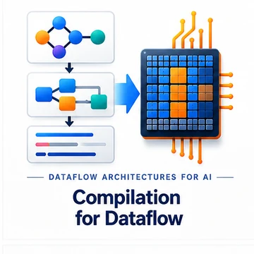
A PyTorch model passes through several compiler stages before it runs, and each stage changes what the hardware executes. The course follows the PyTorch 2 path through TorchDynamo, AOTAutograd, and TorchInductor, then compares fusion, tiling, layout, and scheduling in Inductor with Triton, XLA on TPUs, and the Spyre compiler stack.

Lab: Benchmark eager and compiled execution, inspect a captured graph, repair a graph break, and connect compiler artifacts to the code your run produced.

  • Trace the PyTorch 2 compilation path from TorchDynamo through TorchInductor.
  • Find and fix graph breaks and diagnose recompilation in compiled models.
  • Compare fusion, tiling, layout, and scheduling decisions across Inductor, XLA, and Spyre.
View on Coursera
Memory Systems in Dataflow Architectures course logo
Course 4 5 to 5.5 hours

Memory Systems in Dataflow Architectures

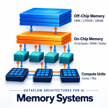
In LLM inference, moving data often takes longer than computing on it. The course explains why low-batch decode is bandwidth-bound, compares hardware-managed caches with compiler-managed local memories, and then covers the KV cache in depth: sizing, MHA and GQA, PagedAttention, prefix caching, chunked prefill, and tiered storage.

Lab: Measure decode time and memory use on a Colab GPU across batch sizes and context lengths, compare them with analytical predictions, and explain the gap.

  • Explain why low-batch decode is often bandwidth-bound and estimate its arithmetic intensity.
  • Compare caches, scratchpads, and on-chip SRAM across accelerator architectures.
  • Size the KV cache and evaluate serving techniques that reduce or manage its memory cost.
View on Coursera
Debugging Across the Dataflow Stack course logo
Course 5 4.5 to 5 hours

Debugging Across the Dataflow Stack

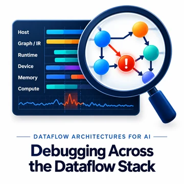
When a compiled model returns a wrong answer, the error often appears far from the operation that caused it. The course organizes failures into eight layers from Python source to hardware, and uses differential debugging, backend ablation, compiler IR, logs, and kernel replay across PyTorch/Inductor, JAX/XLA, and torch-spyre.

Lab: Diagnose three planted failures: an injected NaN, a recompile storm, and a silent numerical divergence. For each one, name the layer and record the evidence.

  • Locate failures in compiled AI workloads by compiler stage and software layer.
  • Tell numerical differences from logic bugs using high-precision references and tolerances.
  • Use ablation, provenance, logs, and comparison to find the first point of divergence.
View on Coursera
Performance Modeling and Optimization course logo
Course 6 4.5 to 5 hours

Performance Modeling and Optimization

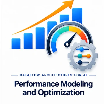
The final course shows how to predict how fast an LLM inference step should run, check the prediction against measurements, and use the difference to find optimizations. It moves from FLOP and byte bounds to PyTorch Profiler traces, benchmarking methodology for compiled code, shape bucketing, and batched decode.

Lab: Measure achieved compute and bandwidth on a GPU, place prefill and decode on a roofline, run a batch sweep, and report time to first token and time per output token.

  • Bound operation runtime from FLOPs and bytes and place workloads on a roofline.
  • Profile LLM decode and separate compute, memory movement, and overhead.
  • Benchmark compiled inference correctly and tune serving shapes from measured evidence.
View on Coursera

How each course works

Video lectures and a graded quiz

Each course is about one week of work. Video lectures run between 1.5 and 2.7 hours per course, and a graded quiz of 16 to 22 questions covers every module.

A 90-minute Colab lab

Every course has a hands-on lab in Google Colab with PyTorch and open-source tools, followed by a 10-question lab quiz. The labs measure real behavior, such as decode time across batch sizes or the cost of a graph break.

One map across six courses

Learners start an Accelerator Landscape Map in the first lab and add to it in each course. By the end it records how each architecture handles execution, memory, and scheduling, and it can be reused to evaluate new hardware.

Optional practice on IBM Spyre

Optional Dataflow Deep Dive activities extend selected labs to IBM Spyre hardware, for learners in partnered programs.

Learners who complete all six courses receive a professional certificate in AI Systems Performance Engineering.

Thank you to Dr. Rashed Bhatti, senior technical staff member at IBM Research, who tested the labs and enhanced several of them.

Start the specialization

You can enroll in the full specialization or start with The Accelerator Landscape. Scan the code with a phone camera, or use the link.

QR code that opens the Dataflow Architectures for AI specialization on Coursera