Why Quantization Won, and Where Pruning Survived: A Practitioner's View of LLM Compression

A practitioner's view of model compression for LLM inference.

I hear the same question from my students at Columbia and from engineers building inference stacks:

If both quantization and pruning compress models and speed up inference, which one do people actually use when they ship an LLM to production?

The short answer: quantization, almost always. Pruning has not disappeared, but production pruning today looks nothing like the unstructured "zero out small weights" approach most textbooks still teach.

The reasons quantization took over are also the reasons pruning has shifted into the specific forms covered later in this post.

1. Why quantization became the default

Every production LLM serving stack today, vLLM, TensorRT-LLM, SGLang, and llama.cpp [6], follows the same recipe. Weights are stored in INT4 or INT8. Many deployments run the whole forward pass in FP8. DeepSeek-V3 trained its forward and backward GEMMs in FP8 from step zero, with higher-precision retention for the numerically sensitive components [1]. The convergence is not accidental.

One distinction matters for the rest of this post. Quantization in practice splits into two very different workflows:

Post-training quantization (PTQ) is applied after a model has finished training. You take the finished FP16 or BF16 checkpoint, run a small calibration dataset through it (a few hundred samples is often enough), estimate the right scaling factors, and write out a lower-precision copy of the weights. No gradient updates, no training infrastructure. GPTQ [7], AWQ [8], and SmoothQuant [9] are the methods most people reach for.

Quantization-aware training (QAT) is applied during training. Low-precision operations are simulated (or performed natively) on the forward and backward passes, so the model's weights adapt to the precision loss as they learn [15]. QAT preserves more accuracy at very low bit-widths, but it costs a training run. For a trillion-parameter model, that cost is enormous.

A third variant has emerged more recently: native low-precision training, where the model is trained end-to-end in FP8 from step zero [1]. This is not exactly QAT, the forward pass is not simulating quantization, it is the quantized computation, but it lives on the same side of the PTQ/QAT divide.

The hardware is on its side. Modern accelerators, H100, Blackwell B200, MI300X, have dedicated low-precision paths. FP8 tensor cores across all three. Blackwell adds native FP4. INT4 weight-only quantization is the common pattern on H100 and MI300X, where weights are stored at 4 bits and dequantized to FP8 or FP16 for compute. These are not afterthoughts. They are designed into the chip because the chip designers knew where the workload was going. Every bit of precision you strip from your weights gives you a direct throughput gain on hardware that is waiting for exactly that.

Generating a token is memory-bound, not compute-bound. My students always underestimate this part. When you generate text one token at a time, you are not bottlenecked by math. You are bottlenecked by how fast you can stream the weights from HBM into the compute units. Cutting weights to 4 bits roughly quarters the memory traffic. That near-quarter translates directly into faster responses [14].

PTQ is cheap, and it works well enough. This last point is the one that decides most production deployments. GPTQ [7], AWQ [8], and SmoothQuant [9] take a finished model and produce a quantized version in hours on a single node. No training data. No gradient updates. For trillion-parameter models where a full training run costs millions of dollars, that gap is enormous. PTQ is the rare optimization that is free in the dimension that hurts most. QAT and native low-precision training exist for the cases where PTQ is not accurate enough, typically INT4 at aggressive settings, or FP8 end-to-end training. But for the bulk of deployments, PTQ is the path of least resistance and the best ROI.

Modern accelerators ship with first-class low-precision paths: FP8, INT8, and INT4 kernels are designed into the silicon. Unstructured sparsity has no matching hardware path, and even 2:4 structured sparsity gives only a limited speedup on the sparse tensor cores it can target.

2. Why pruning stalled for LLMs

Pruning has a longer history than quantization in deep learning. It worked well for vision models. It produced beautiful lottery ticket papers. So why did it not follow the same trajectory for LLMs?

Zeros that hardware cannot skip are not actually free. If you zero out 50% of a weight matrix at random, a standard GPU will still multiply by those zeros. You saved memory on paper, if you compressed the storage format, but the math still runs. This is the core problem. Unstructured sparsity is a statement about the model. Speedup is a statement about the hardware. Without a bridge between them, pruning gives you a smaller file and nothing else.

2:4 semi-structured sparsity is the real bridge, and it is narrow. NVIDIA Ampere and newer GPUs have sparse tensor cores that can exploit a very specific pattern: in every group of four weights, at least two must be zero [16]. Force your model into that pattern, and you get around a 1.5× to 1.7× speedup on the sparse kernel paths. The problem is that enforcing 2:4 usually needs fine-tuning to recover accuracy, and fine-tuning a trillion-parameter model is not a one-afternoon job.

One-shot methods closed part of the gap. SparseGPT [17] and Wanda [18] made it possible to prune LLMs without retraining, a real achievement, and conceptually analogous to PTQ for quantization. But "possible" is not the same as "worth it." When PTQ quantization gives you 4× memory savings with a few hours of calibration, and one-shot pruning gives you 1.5× speedup (and only if you meet the 2:4 pattern constraint, often after additional fine-tuning), the choice is clear.

3. The roofline picture that makes all of this obvious

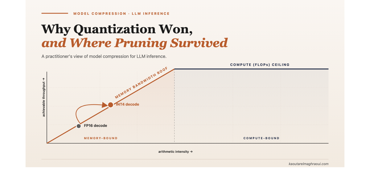
The clearest way to see this is a roofline plot [14].

Looking at the roofline model of an LLM decoding workload, we can see that token generation lives in the memory-bound region, far to the left of the compute ceiling. Quantization acts on the horizontal axis: it shrinks the bytes moved per operation and lifts achievable throughput directly. Pruning, unless the hardware can skip the zeros, does nothing to this picture.

LLM decoding sits in the memory-bound region. The bottleneck is bandwidth, not FLOPs. Quantization directly helps bandwidth by storing fewer bits per weight, which means fewer bytes have to move on every token. Pruning, on its own, does not shift you off the memory roof unless the hardware can translate sparsity into skipped memory reads. Most cannot.

Once you see this, the question stops being which technique is better. It becomes which bottleneck each technique targets. That is the right question to ask.

4. Where pruning still lives

Pruning did not disappear. It shifted. In modern inference stacks, you will find four use cases where pruning is still applied.

Four forms of sparsity matter in today's LLM inference stacks. Each one found a way to align with the hardware, either by producing a smaller dense model, or by reducing memory traffic in a pattern the hardware can exploit.

Structured pruning, to produce smaller dense models. Work like Sheared LLaMA [13], LLM-Pruner [19], and NVIDIA's Minitron [4] [5] prunes whole heads, whole channels, or whole layers. The output is a smaller dense model that runs on ordinary tensor cores with no special kernels required. You then quantize the smaller model on top. This is the one place where classical pruning is thriving in LLM deployment.

KV cache compression. During long-context inference, the memory pressure is not in the weights, it is in the KV cache, which grows with sequence length. Methods like H2O [10], Scissorhands [20], and SnapKV [11] drop less-important tokens from the cache as generation proceeds. This is pruning along the sequence dimension, at serving time. For long-context deployments, it is often the single most impactful memory optimization available.

Activation sparsity. Many neurons in the feed-forward layers do not fire for a given token. Approaches like Deja Vu [12] detect which neurons will be inactive and skip them dynamically. This is fine-grained dynamic sparsity, and it works because the pattern is predictable enough to route around in software.

Mixture of Experts. The most successful form of sparsity in modern LLMs, even though we rarely call it pruning. MoE activates only a subset of experts per token. The rest of the model sits idle. DeepSeek-V3 [1], Mixtral [21], GPT-OSS [22], all are MoE architectures. Sparsity at the scale and pattern that hardware can route around.

5. How practitioners actually decide

In my experience, the real decision is never "quantization or pruning." It is a layered recipe.

Modern LLM deployments use a layered compression recipe in which each stage targets a different bottleneck, and the stages compose rather than compete.

A practitioner shipping an LLM today typically asks three questions in order:

Do I need a smaller model at all? If yes, use structured pruning or distillation [4] [5] to shrink a bigger model into a smaller dense one. This is the expensive step, and it is only worth it when you know you need the smaller footprint for a specific hardware target.

What precision can I quantize to, and can I do it post-training? This is almost always a PTQ question. INT8 weights are nearly always safe with PTQ. INT4 with good calibration, GPTQ [7] or AWQ [8], is usually safe for chat and retrieval workloads without retraining. SmoothQuant [9] handles activation quantization when weight-only isn't enough. QAT enters the picture only if PTQ does not hold up at the precision you need, which in 2026 is rare for INT8 and increasingly rare for INT4 thanks to calibration-aware methods. Native FP8 training (as in DeepSeek-V3 [1]) is still mostly something frontier labs do during pretraining, not something most teams retrofit. PTQ is the cheapest and highest-leverage step, so it is almost never skipped.

Is long-context memory my bottleneck? If yes, add a KV cache compression method at serving time [10] [11]. This is orthogonal to the weight-compression decisions above.

Unstructured pruning is missing from this list. In production, stacking it with quantization is rare. The complexity does not pay for itself when quantization alone captures most of the win.

6. Four case studies from real deployments

The recipe above is abstract. Four recent deployments make it concrete.

DeepSeek-V3, native FP8 training from step zero

DeepSeek-V3 is the clearest example of quantization elevated to a first-class training and inference concern. The model is 671B total parameters with 37B active per token (an MoE design), and it was trained natively in FP8, the first publicly documented frontier-scale model to validate this approach end-to-end [1]. This sits outside both PTQ and classical QAT [15]: the forward and backward passes run in FP8 on Hopper tensor cores from step zero, with strategic high-precision retention for numerically sensitive components (embeddings, normalization, the MoE gate).

The team reports total training cost of 2.788M H800 GPU-hours, with FP8 accelerating GEMMs on Hopper tensor cores and reducing memory pressure throughout. To control FP8's narrow dynamic range, they used fine-grained tile-wise scaling (1×128 for activations, 128×128 for weights) and promoted accumulation to FP32 in CUDA cores [1] [2]. The relative loss delta versus BF16 stayed under 0.25%.

What makes DeepSeek-V3 a good case study is that every compression decision is hardware-aware. FP8 was chosen because H800 tensor cores have an FP8 path. MoE was chosen because gating most of the network off per token reduces both compute and memory traffic. MLA (Multi-head Latent Attention) was added to compress the KV cache. Three different forms of sparsity and low-precision, each aligned with a specific hardware capability.

Llama 4, one model, two deployment paths

When Meta released Llama 4 in 2025, the deployment story split cleanly by model size [3]. Llama 4 Scout (109B total, 17B active) ships with on-the-fly INT4 quantization, effectively PTQ computed at load time, that lets it fit on a single H100 GPU. Llama 4 Maverick (~400B total, 17B active) ships with FP8 weights from training, which fit on a single H100 DGX host, a full 8-GPU node, while preserving quality. Meta reported using FP8 precision during pretraining of the larger Behemoth model at 390 TFLOPs/GPU on 32K GPUs.

The two precisions are chosen for different reasons. INT4 via PTQ maximizes VRAM savings when the constraint is fitting on one GPU. FP8 training preserves more quality when the budget allows a whole node. One is applied after training, the other is part of the training itself. And both are weight-precision stories, there is no unstructured pruning anywhere in Meta's deployment recipe. The sparsity in Llama 4 comes from MoE architecture, not from pruning.

NVIDIA Minitron, structured pruning plus distillation, then PTQ

Minitron is the clearest published example of structured pruning in production. NVIDIA took Llama 3.1 8B and produced Llama-3.1-Minitron-4B by pruning embedding size, attention heads, and MLP intermediate dimension, then running knowledge distillation on the pruned student. The full pipeline includes a teacher-correction step on ~94B tokens of unlabeled data, with the actual distillation on the pruned student using a smaller token budget [4] [5]. Minitron is not a one-shot method like SparseGPT [17] or Wanda [18]. The pruning step is followed by a real (albeit shortened) training pass that lets the smaller architecture recover what it lost. The result is a dense 4B model that runs on ordinary tensor cores and fits smaller hardware envelopes, no sparse kernels required, no special runtime support.

The numbers are telling. Compared to training a 4B model from scratch, Minitron needed roughly 40× fewer training tokens and delivered about a 16% improvement in MMLU [4]. Producing the full Nemotron-4 family (15B, 8B, 4B) via pruning and distillation instead of independent training runs cut total compute cost by ~1.8× [5]. The community then applied PTQ FP8 quantization on top of the pruned checkpoints, yielding FP8 variants of Minitron on Hugging Face [4]. This is the production recipe playing out exactly as described: structured prune → distill → PTQ quantize.

llama.cpp and GGUF, PTQ is what enables local LLMs

If you run an LLM on a laptop, a phone, or a Raspberry Pi, you are almost certainly using a GGUF (GPT-Generated Unified Format) file and llama.cpp [6]. GGUF is the binary file format used by llama.cpp to package quantized model weights, tokenizer, and metadata into a single self-contained file that can be memory-mapped on consumer hardware. The entire GGUF ecosystem is a PTQ ecosystem: the community takes a released FP16 checkpoint, runs it through llama-quantize with a chosen format, optionally computes an importance matrix to protect sensitive layers, and ships the result. No retraining, no training framework, no gradients. GGUF supports 1.5-bit through 8-bit integer quantization, with the Q4_K_M mixed-precision format emerging as the practical default, roughly 40 GB for a 70B-class model, which fits a single high-end consumer machine with unified memory [7]. Apple Silicon is treated as a first-class target, with ARM NEON, Accelerate, and Metal backends [6].

There is no pruning in this ecosystem at all. The entire on-device LLM revolution rides on PTQ quantization, importance matrices (so that sensitive layers like attention projections keep more bits), and efficient kernels that work well on consumer hardware. When Apple Intelligence, Gemma, and Phi-3 run on phones, they run because quantization made them small enough to fit, not because anyone pruned them.

7. The question worth asking

Compression is often taught as a menu of independent techniques, like a choice between A and B. In production, it is hardware-bound: a technique only delivers real speedup when the silicon can exploit the sparsity or precision pattern it produces.

Quantization won because its pattern, fewer bits per weight, aligns with how modern accelerators are built and where LLM inference spends its time. Pruning, in the forms that survived, learned the same lesson the hard way. Produce a smaller dense model that standard hardware can run, or compress along a dimension (KV cache, experts, activations) the hardware already knows how to skip.

The research-paper framing of "pick one technique" does not match how real systems work. Real systems layer techniques together, and the layering is driven by where the bottleneck is. For autoregressive LLM inference, that is almost always memory bandwidth.

So the question I would ask, every time, is not which compression technique should I use. It is what is the bottleneck, and which technique shifts it? The rest follows from there.

That is also the thing I keep telling my students. The methods will keep changing. The bottleneck question won't.

---

References

[1] DeepSeek-AI, "DeepSeek-V3 Technical Report," arXiv:2412.19437, December 2024.

[2] DeepSeek-AI, "Insights into DeepSeek-V3: Scaling Challenges and Reflections on Hardware for AI Architectures," Proceedings of the 52nd Annual International Symposium on Computer Architecture (ISCA), 2025.

[3] Meta AI, "The Llama 4 herd: The beginning of a new era of natively multimodal AI innovation," Meta AI Blog, April 2025.

[4] Muralidharan, S. et al., "Compact Language Models via Pruning and Knowledge Distillation," arXiv:2407.14679, July 2024.

[5] Sreenivas, S. T. et al., "LLM Pruning and Distillation in Practice: The Minitron Approach," arXiv:2408.11796, August 2024.

[6] ggml-org, "llama.cpp — LLM inference in C/C++," GitHub repository.

[7] Frantar, E. et al., "GPTQ: Accurate Post-Training Quantization for Generative Pre-trained Transformers," ICLR 2023.

[8] Lin, J. et al., "AWQ: Activation-aware Weight Quantization for LLM Compression and Acceleration," MLSys 2024.

[9] Xiao, G. et al., "SmoothQuant: Accurate and Efficient Post-Training Quantization for Large Language Models," ICML 2023.

[10] Zhang, Z. et al., "H₂O: Heavy-Hitter Oracle for Efficient Generative Inference of Large Language Models," NeurIPS 2023.

[11] Li, Y. et al., "SnapKV: LLM Knows What You are Looking for Before Generation," NeurIPS 2024.

[12] Liu, Z. et al., "Deja Vu: Contextual Sparsity for Efficient LLMs at Inference Time," ICML 2023.

[13] Xia, M. et al., "Sheared LLaMA: Accelerating Language Model Pre-training via Structured Pruning," ICLR 2024.

[14] Williams, S., Waterman, A., Patterson, D., "Roofline: An Insightful Visual Performance Model for Multicore Architectures," Communications of the ACM, 2009.

[15] Jacob, B. et al., "Quantization and Training of Neural Networks for Efficient Integer-Arithmetic-Only Inference," CVPR 2018.

[16] Mishra, A. et al., "Accelerating Sparse Deep Neural Networks," arXiv:2104.08378, 2021.

[17] Frantar, E., Alistarh, D., "SparseGPT: Massive Language Models Can Be Accurately Pruned in One-Shot," ICML 2023.

[18] Sun, M. et al., "A Simple and Effective Pruning Approach for Large Language Models (Wanda)," ICLR 2024.

[19] Ma, X. et al., "LLM-Pruner: On the Structural Pruning of Large Language Models," NeurIPS 2023.

[20] Liu, Z. et al., "Scissorhands: Exploiting the Persistence of Importance Hypothesis for LLM KV Cache Compression at Test Time," NeurIPS 2023.

[21] Jiang, A. Q. et al., "Mixtral of Experts," Mistral AI, arXiv:2401.04088, January 2024.

[22] OpenAI, "Introducing gpt-oss," open-weight Mixture-of-Experts models, August 2025.