Decision Models: A New Breed, or a Systems Correction?

A customer support system has to decide whether to answer a ticket, escalate it, or ask for more information. That is three options. Running a model that writes a paragraph, which the code then parses back into one of those three labels, is more work than the task needs. The new "decision models" answer the typed question directly. TypeSafe's Jev named the category "System One models," and within weeks Cloudflare and others shipped their own. I covered the launch on IBM's Mixture of Experts podcast. This is what these models are, where they help, and why I read the category as a systems correction built from methods the field already had.

What decision models return

A generative model answers a yes/no question by writing the word "yes" one token at a time, and the code parses that text back into a value. A decision model returns the value directly. You give it the current state, a typed question, and the set of allowed answers, and it returns one of those answers with a probability attached. TypeSafe describes Jev's output as "typed probabilistic decisions," with choices up to a cardinality of 255, and reports end-to-end response times of 70 to 500 milliseconds. Those are vendor figures, reported without percentiles or test conditions [1].

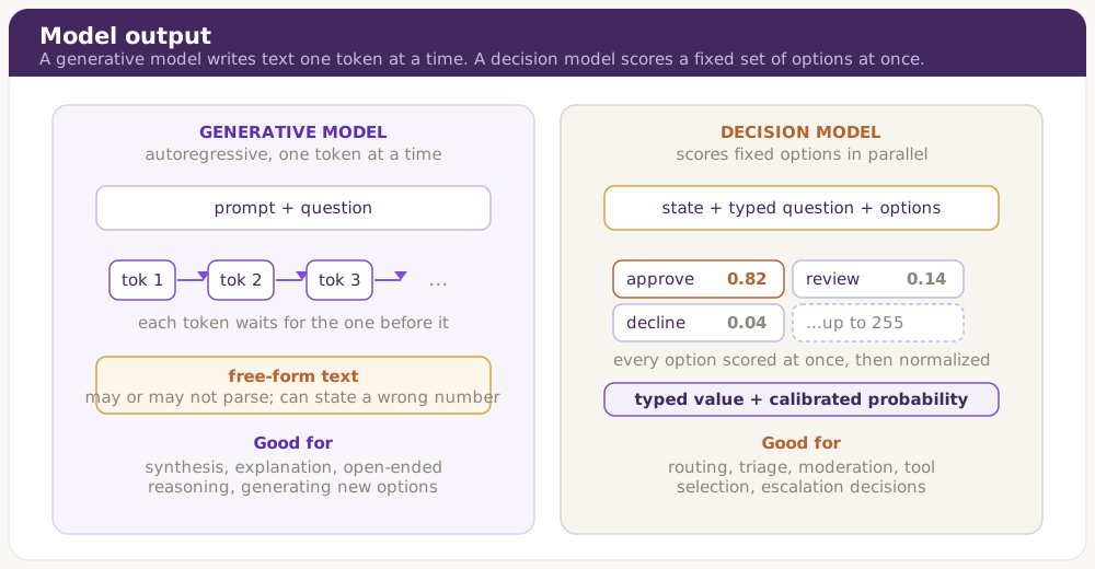
Fig. 1 — A generative model writes text token by token, and the code parses it. A decision model returns a typed value the software can act on directly. The probability is an estimate, not a guarantee of correctness.

The useful part is that the output becomes a value the software can act on directly, without parsing prose first. One caveat up front, because it runs through the rest of this piece. A typed output, a calibrated probability, and a correct decision are three separate things. A model can give you the first without the second, and the second without the third. I will keep them separate throughout.

Several ways to implement a decision

"Decision model" is a product label. It describes an interface, not a specific architecture. A bounded output can be produced in at least four ways, and they differ in cost, flexibility, and what the probability means.

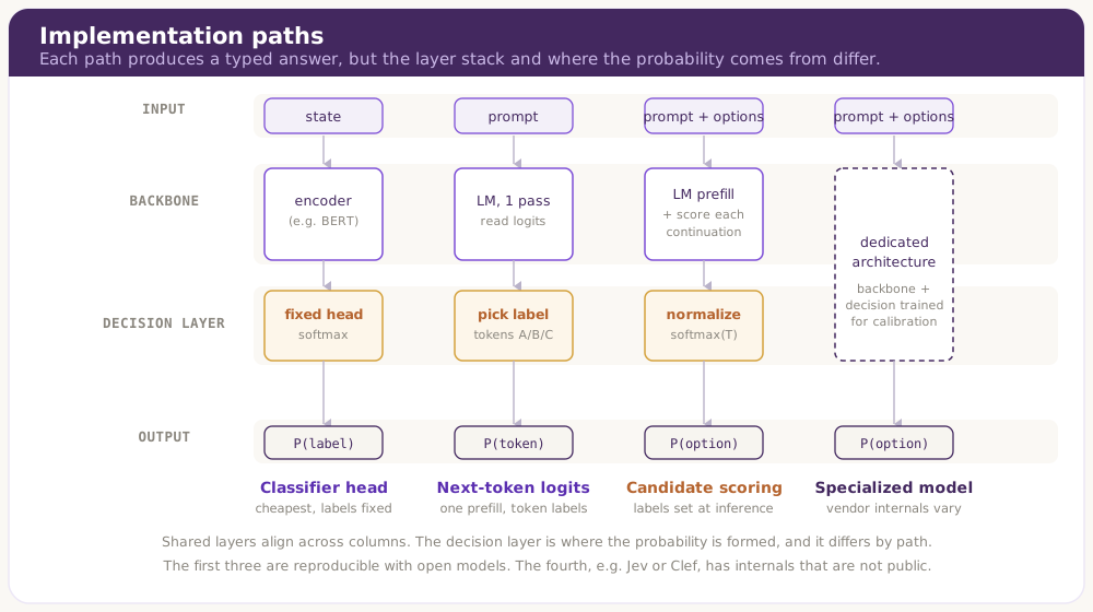
Fig. 2 — Four ways to produce a bounded decision. They return the same shape of answer but differ in compute, tokenization behavior, and how their probabilities should be read. A product's public interface does not tell you which path it uses.

A trained classifier puts a fixed label head on a learned representation. It is the cheapest and the least flexible, because the labels are set at training time. Next-token scoring reads the model's logits for preselected single-token labels after one prefill pass. It is fast, and it is sensitive to tokenization and label wording. Candidate scoring appends each full option to a shared prompt and scores the continuation, so the labels can be defined at inference time, at the cost of more work as the number of options grows. A specialized model, which is what the vendors ship, uses its own architecture, training, and serving stack, and its internals are not public.

One open reproduction works through the candidate-scoring path in detail, and it is the clearest public account of how this can be done [2]. The model completes a sentence rather than answering freely. It reads the prompt once, in parallel, because every token of the prompt is known in advance. It then scores each allowed option by appending it and reading the probability the model assigns to that continuation, and it normalizes the scores so they sum to one.

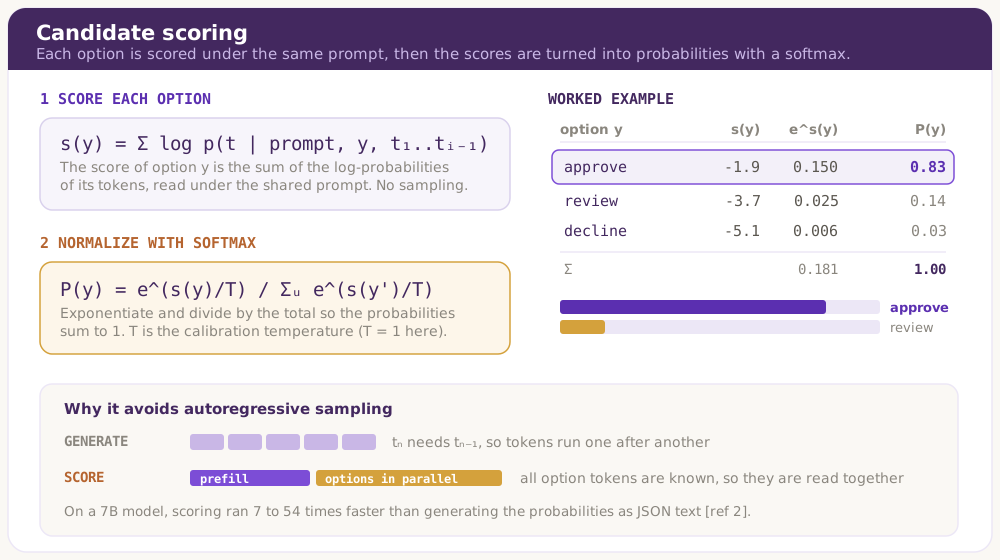
Fig. 3 — One documented way to implement a decision, candidate-continuation scoring. This is not a claim about any proprietary model's internals.

Two points are worth stating precisely, because the launch coverage blurred both. First, knowing the candidate tokens in advance avoids autoregressive sampling, but it does not avoid the computation. Each option's tokens still contribute work, evaluated in parallel with causal masking rather than generated one at a time. TypeSafe's "one forward pass" is a product-level simplification. The documented path is closer to a prefill pass plus a scoring pass, and the exact count is an implementation detail. Second, normalizing over the supplied options gives a probability mass over those options. It is not a probability that the answer is correct in the world. If the right answer is not in the set, the model still returns a confident choice from the wrong set.

The speed argument still holds in the right direction. Generating an answer is serial, because the step that predicts token 302 needs token 301, which does not exist until the previous step ran. Scoring avoids that dependency. In the same reproduction, on a 7-billion-parameter model, scoring ran 7 to 54 times faster than generating the probabilities as JSON text, with the exact ratio depending on output length and setup [2]. One baseline the launch posts skipped is worth naming. A generative model with grammar or JSON-schema-constrained decoding also guarantees a valid, in-set answer, so guaranteeing valid output is not on its own what sets a decision model apart. Any real advantage has to show up in latency, probability quality, or cost.

Calibration decides whether you can trust the number

The appeal of a decision model is that your software can treat the probability as a real quantity, routing anything above 0.9 automatically and escalating the rest. That only works if the probability is calibrated. Calibration is a distinct property from validity and accuracy, and it has to be checked on its own.

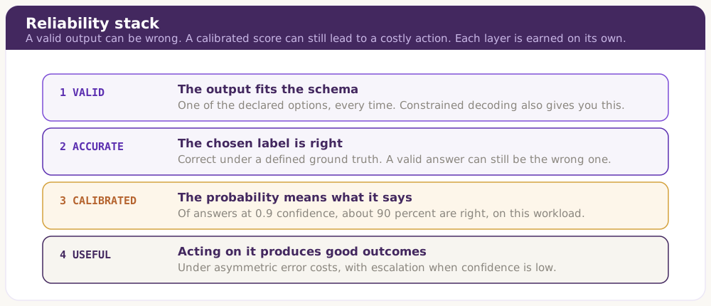
Fig. 4 — Validity, accuracy, calibration, and decision utility are four separate requirements. A valid output can be wrong, and a calibrated model can still make a costly mistake.

A model is calibrated when its confidence matches its accuracy. Of a thousand answers at 90 percent confidence, about 900 should be right. Models are not calibrated by default. In that reproduction, instruction-tuned models were badly overconfident. At 77 options, a 7-billion-parameter instruct model averaged 95 percent confidence while being right 64 percent of the time [2]. Correcting this takes work. Temperature scaling, which divides every score by one fitted number before normalizing, brought that model's expected calibration error from 0.10 to 0.03, and it needs labeled examples from your own task to fit that number [2]. TypeSafe trains for calibration with an unpublished method it calls Reinforcement Learning for Calibrated Decisions [1], and Cloudflare's open Clef models add a Brier-score term to the training loss for the same purpose [3].

Two metrics appear here, and they measure different things. Expected calibration error, ECE, is a binned summary of the gap between confidence and accuracy. Its value depends on the binning, and it can hide a subgroup that fails. The Brier score is a proper scoring rule that measures mean squared probabilistic error, so it rewards probabilities that are both calibrated and sharp. None of this is new. Modern networks are known to be overconfident, and temperature scaling and reliability diagrams are standard tools for diagnosing it [5]. For anything high-stakes, report ECE and the Brier score together, with reliability plots and class-wise checks, rather than one summary number.

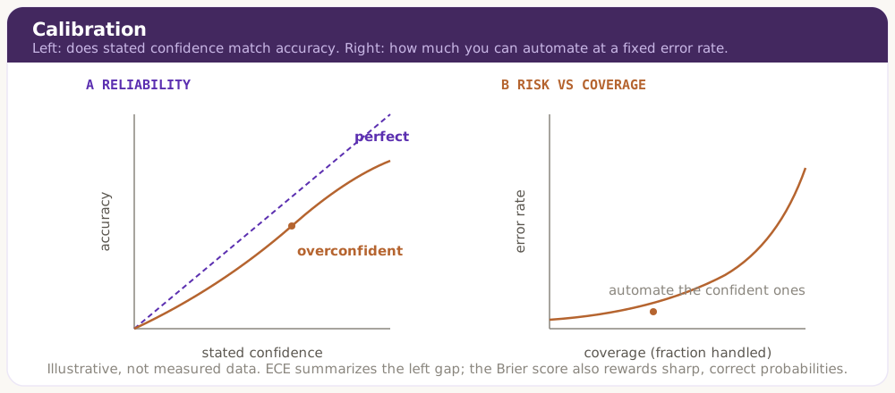
Fig. 5 — Calibration asks whether a stated probability means what it says, and selective prediction asks how much you can automate at a fixed error rate. Shapes are illustrative, not measured.

The point that matters most in deployment is that calibration does not transfer across tasks. An independent benchmark found Jev well calibrated on its target tasks, with ECE around 0.033, and 0.251 when pooled across social-science tasks it was not tuned for. Fitted temperatures also failed to carry across different option counts [4]. The practical approach is selective prediction. Pick a confidence threshold, automate what clears it, escalate the rest, and measure the error rate on the part you automate. Recalibrate on your own data and option set before you trust any threshold.

When the question changes the answer

Developers tend to treat labels and schemas as fixed metadata that the model ignores. For a prompt-conditioned decision model, the labels are part of the input. The output can change when you edit them in ways that should not matter, such as reordering or rewording them.

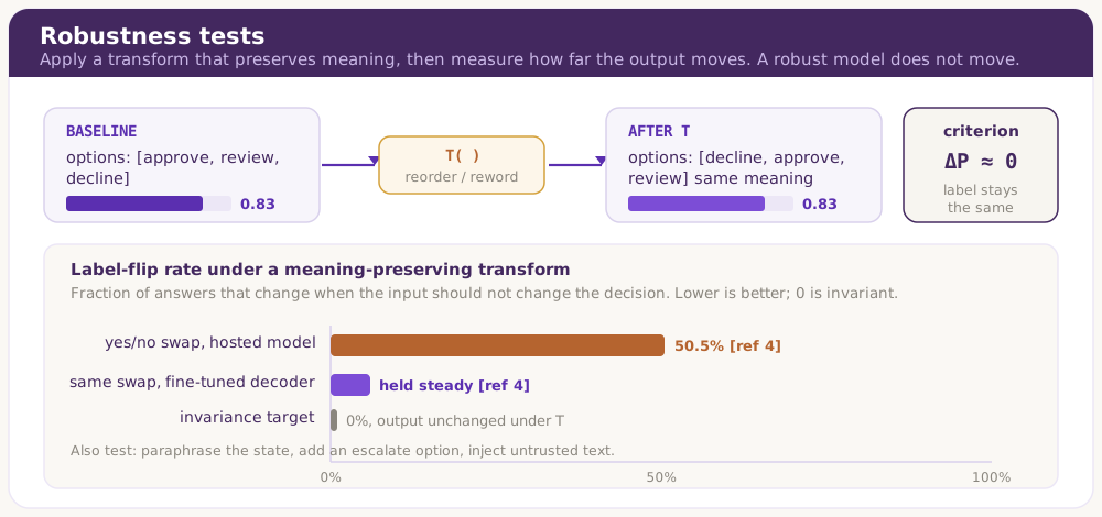
Fig. 6 — A stable interface shape does not imply stable behavioral semantics. Test under changes that preserve meaning, and note separately when a change genuinely alters the decision problem.

The same benchmark makes this concrete. Swapping the yes and no options flipped about half of the hosted model's answers, 50.5 per hundred, while fine-tuned decoder checkpoints held steady through the swap [4]. So a robustness test suite is worth running. Shuffle the option order and watch the chosen label and its probability. Paraphrase the state and the labels without changing their meaning. Add an escalate option, and note that this can genuinely change the decision problem, so read that result separately. When the input state carries untrusted text, run prompt-injection tests. A typed output constrains the shape of the answer. It does not tell you whether the answer was manipulated.

Costing the whole decision workflow

A cheap model call can still produce an expensive system. A wrong route triggers retries, human intervention, customer harm, or downstream rework, and those costs dwarf the inference. The quantity worth optimizing is the cost of the whole workflow, measured per decision that succeeds, not the latency of a single inference.

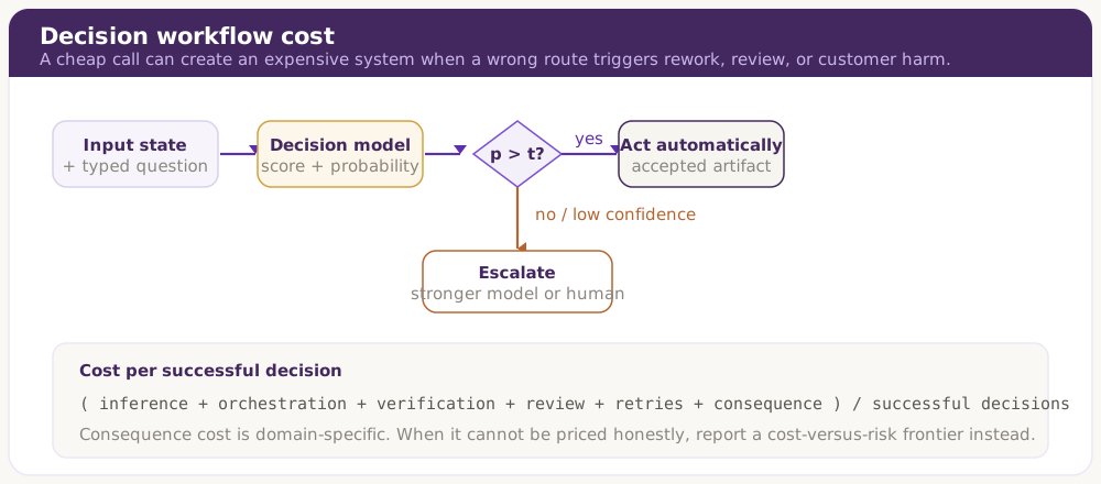
Fig. 7 — The useful objective is cost per successful decision across the whole path, not tokens per second at the model. Consequence cost is domain-specific, so report a cost-versus-risk frontier when it cannot be priced honestly.

A real deployment comparison needs several candidates on the same task, not one model. Put a dedicated classifier, an embedding model with logistic regression, a prompted decision model, a generative model with constrained decoding, a generative model read through option scoring, and a cascade that sends cheap first-stage decisions to a stronger model or a human only when needed. Measure p50, p95, and p99 latency at target load, dollars per thousand inputs, accuracy or macro-F1, calibration, the error rate at a fixed coverage, and the human-escalation rate. In that benchmark the cascade did well. An intent-trained first stage that escalated to Jev matched Jev's accuracy at 0.43 of its cost [4].

What the accelerator executes

This is the part I want to be clearest about, from the systems side, because the launch coverage skipped it. The hardware does the same kind of work whether the answer is a sentence or a Boolean. It executes operations and moves bytes. The efficiency gain comes from changing the computation needed to produce the answer, and the output format alone does not change that computation.

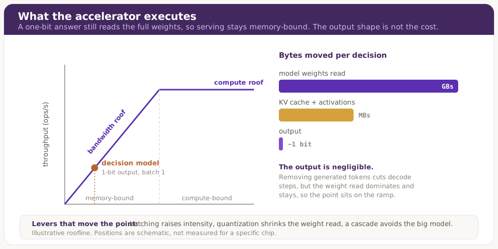
Fig. 8 — A decision model stays on the memory-bound ramp of the roofline even for a one-bit output, because the weight read dominates the bytes moved. Batching, quantization, and cascades move the operating point; the output shape does not. The roofline is illustrative, not measured for a specific chip.

Several consequences follow. A large model can stay memory-bandwidth-bound even when it returns one bit, because serving still has to move the weights, so measure bytes moved and cache residency rather than output length. Removing multi-token generation does cut sequential decode steps, but it does not remove the prompt prefill or the candidate-scoring work. A fixed output schema can help the scheduler batch requests, though variable input lengths, changing option counts, and latency deadlines complicate the batching. Quantization can lower cost, and it shifts the logits, so probability reliability has to be rechecked after quantizing, not only top-1 accuracy. At low utilization a specialized model can be faster per request and still more expensive per decision than a small classifier with a fallback. So the gains to chase are in batching, precision, and model size, which is where the computation actually changes.

Where the category actually fits

A decision model earns its place when the task is a genuine choice from a fixed set, when you do not already have labeled data to train a classifier, and when latency or cost per decision makes autoregressive generation wasteful. Intent routing, content triage, moderation, tool selection, and escalation all fit. The benchmark supports this placement. When labels were available, a small trained classifier still won on intents: a fine-tuned BERT-base reached 0.940 and logistic regression on embeddings reached 0.948, against Jev's 0.913 on the same CLINC-150 accuracy measure. Without labels, a zero-shot classifier fell to 0.507, and the decision model landed usefully between the two [4]. A generative model read through option scoring matched the hosted decision model on both tasks, which indicates the gains come from the scoring technique and the calibration training rather than from a new kind of model [4].

My take, from the systems side

We have been paying a generative-model tax on decisions that were always typed, running a model that writes paragraphs to produce a yes or a no. Decision models remove that overhead, and the correction is real. The useful unit of engineering is the whole path from input to action: the model, its uncertainty, the decision policy, the fallback, and the outcome you measure. Underneath "System One" is a learned conditional decision function, the probability of an answer given the state, the question, and the options, built with scoring and calibration methods the field already had. That is an advance in packaging and discipline. It is not a new form of intelligence.

The vendor numbers deserve the scrutiny any vendor numbers get. TypeSafe is candid that its headline comparisons ran under conditions favorable to its model, that its reference answers bias toward two specific model families, and that it cannot prove its pricing is not subsidized [1]. That candor is to its credit, and it is the reason to run your own evaluation.

Decision models give software a more direct way to ask for a judgment, and for the right workloads that is better than generating text and parsing it back. A valid output can still be wrong, and a calibrated model can still make a costly mistake. So the category is worth adopting where it fits, and worth measuring end to end before you do. That is the engineering, and it has not changed.

---

References

[1] TypeSafe AI, "Introducing System One Models and Jev," 2026.

[2] V. Dibia, "How Jev works: calibrated decision models," 2026. Open reproduction of candidate-continuation scoring on Qwen2.5 models; invalid-JSON rates, 7 to 54x scoring speedup, and ECE figures are from this work.

[3] Cloudflare, "Introducing Clef: our open-source decision models, and new RL fine-tuning platform," 2026.

[4] "Benchmarking System One decision models against trained classifiers and language models for automated decision gates," arXiv:2610.00346, 2026. Source for the classifier and zero-shot accuracy figures, the yes/no swap sensitivity, the pooled-task ECE, and the cascade cost result.

[5] C. Guo et al., "On Calibration of Modern Neural Networks," ICML 2017. Background on calibration, reliability diagrams, ECE, and temperature scaling.